Instructions: this week’s exercise is called 3_hhi.R. Download or copy-paste that file into a new R script, then open it and run it with the working directory set as the IDA folder. If you download the script, make sure that your browser preserved its .R file extension.
The rest of this page documents the exercise and expands on what you learn from it.
The exercise shows how to compute market concentration for Internet browsers by writing a Herfindhal-Hirschman Index (HHI) function, and also shows you how to defend that function against bad input. The HHI function written in the exercise will eventually contain comments and defensive statements. It will look like this:
# HHI function.
hhi
function(x, normalized = FALSE) {
    # check argument
    if(!is.numeric(x)) stop("Please provide a numeric vector of values")
    # check percentages
    if(sum(x) == 100) {
        message("Percentages converted to fractions")
        x <- x / 100
    }
    # check sum
    if(sum(x) != 1) warning("Shares do not sum up to 1")
    # sum of squares
    hhi <- sum(x^2)
    # normalize if asked
    if(normalized) {
        message("HHI normalized to [0, 1]")
        hhi <- (hhi - 1 / length(x)) / (1 - 1 / length(x))
    }
    # send back result
    return(cat("HHI =", hhi, "\n"))
}
The actual formula for the Herfindhal-Hirschman Index is \(HHI =\sum_{i=1}^N s_i^2\) where \(s\) is the usage share of each of \(N\) browsers: it's a sum of squared market shares, with applications to any market and to other things like political parties.
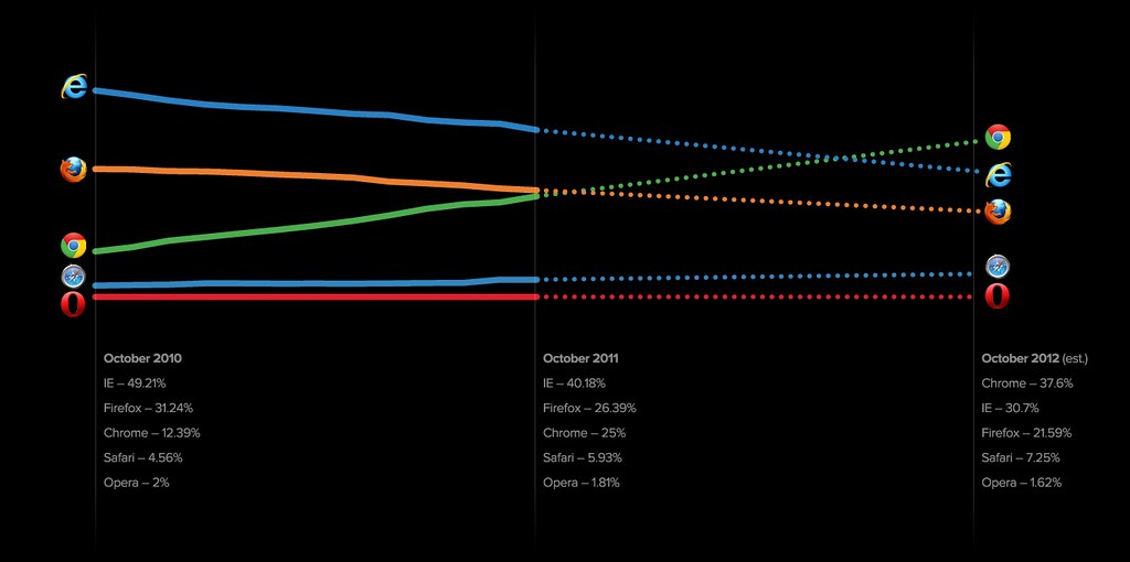
We can expand on that example by using historical data from StatCounter, a company that tracks browser usage worldwide. Here's what this market has looked like in recent years:
Data from 2008 to 2013 can be collected from Wikipedia with a little help from the XML package to read the HTML-formatted data from Wikipedia. The following packages are required:
# Load packages.
require(ggplot2)
require(reshape)
require(XML)
The next code block anticipates on next week's session: it downloads and converts data from a Wikipedia table, and then saves it to a plain text file. Many thanks to Juba for a slight optimization in the data cleaning routine, at the point where we use the gsub() function to remove percentage symbols from the values.
# Target file.
file <- "data/browsers.0813.csv"
# Load the data.
if (!file.exists(file)) {
    # Target a page with data.
    url <- "http://en.wikipedia.org/wiki/Usage_share_of_web_browsers"
    # Get the StatCounter table.
    tbl <- readHTMLTable(url, which = 16, as.data.frame = FALSE)
    # Extract the data.
    data <- data.frame(tbl[-7])
    # Clean numbers.
    data[-1] <- as.numeric(gsub("%", "", as.matrix(data[-1])))
    # Clean names.
    names(data) <- gsub("\\.", " ", names(data))
    # Normalize.
    data[-1] <- data[-1]/100
    # Format dates.
    data[, 1] <- paste("01", data[, 1])
    # Check result.
    head(data)
    # Save.
    write.csv(data, file, row.names = FALSE)
}
The data can now be loaded from the hard drive and prepared for analysis. Our first step is to convert dates to proper date objects, which will avoid plotting issues. This process uses time code format for day-month-year, %d %B %Y, where %d is the day of month, %B the full month name and %Y the year with century. This process is explored again when we get to time series in Session 9.
# Load from CSV.
data <- read.csv(file)
# Convert dates.
data$Period <- strptime(data$Period, "%d %B %Y")
# Check result.
head(data)
      Period Internet.Explorer Chrome Firefox Safari  Opera
1 2013-05-01            0.2914 0.3839  0.2119 0.0986 0.0113
2 2013-04-01            0.3057 0.3712  0.2136 0.0948 0.0122
3 2013-03-01            0.3192 0.3583  0.2129 0.0952 0.0121
4 2013-02-01            0.3310 0.3457  0.2140 0.0951 0.0121
5 2013-01-01            0.3567 0.3279  0.2079 0.0941 0.0116
6 2012-12-01            0.3465 0.3268  0.2159 0.0958 0.0131
We now compute the normalized Herfindhal-Hirschman Index, which is \(HHI^* = {\left ( HHI - 1/N \right ) \over 1-1/N }\), with \(HHI =\sum_{i=1}^N s_i^2\) where \(s\) is the usage share of each of \(N\) browsers.
# Normalized Herfindhal-Hirschman Index.
HHI <- (rowSums(data[2:6]^2) - 1/ncol(data[2:6]))/(1 - 1/ncol(data[2:6]))
# Form a dataset by adding the dates.
HHI <- data.frame(HHI, Period = data$Period)
The final plot uses stacked areas corresponding to the user share of each browser, and overlays a smoothed trend of the normalized HHI curve as a dashed line.
# Reshape.
melt <- melt(data, id = "Period", variable = "Browser")
# Plot the HHI through time.
ggplot(melt, aes(x = Period)) + labs(y = NULL, x = NULL) +
  geom_area(aes(y = value, fill = Browser),
            color = "white", position = "stack") +
  geom_smooth(data = HHI, aes(y = HHI, linetype = "HHI"),
              se = FALSE, color = "black", size = 1) +
  scale_fill_brewer("Browser\nusage\nshare\n", palette = "Set1") +
  scale_linetype_manual(name = "Herfindhal-\nHirschman\nIndex\n",
                        values = c("HHI" = "dashed"))

The data manipulations performed here are next week's topic: getting data in and out, and reshaping it to aggregate figures for analysis and plotting.
Next week: Data.