Collapsing a bipartite co-occurrence network
This note is a follow-up to the previous one. It shows how to use student-submitted keywords to find clusters of shared interests between the students.
Dear students
If you enjoyed my previous note, this one might also entertain you. And since your real first names are used in the data, you should be able to tell me later if this note makes sense with regards to the true clusters (i.e. student groups) that you formed in my class.
tl;dr – This note explains how to plot this graph in less than 70 lines of code:

The data: Your keywords
Let's start by loading the same dataset that we used to plot a co-occurrence network out of your research interests:
We will start by extracting your first names, which, very conveniently, are unique (there are no duplicate first names in the data):
The result of that operation is simply a vector of your 17 first names in alphabetical order, because we sorted the data on the name when we imported it.
Let's now obtain a vector of all the different keywords that you submitted, following the same separation rule as used in the previous note: keywords separated by a comma or by the "and" conjunction, as in "Sexuality and Gender", will be treated as discrete (separate) entities. The code for that operation is a bit more obscure:
The result of that operation is a vector of 34 alphabetically-sorted keywords, starting with the following ones:
Collective Action, Community Empowerment, Community/Neighborhood, Conflict, ...
We are now going to build a matrix with as many rows as there are students ($n = 17$), and as many columns as there are distinct keywords in the complete data ($k = 34$). The matrix, which will be a non-square, asymmetrical matrix, will serve as the basis for the bipartite (or two-mode) network that we are going to build.
The concept: Bipartite/two-mode networks
A two-mode network is a network in which there are two distinct kinds of entities (modes). These networks are fairly common in the social sciences: just think of a network formed by individuals who are members of groups, such as trade unions, political parties or Facebook groups.
The two different "modes" of a two-mode network are referred to as the "primary" and "secondary" modes. In the case at hand, the primary mode will be you, the students, and the secondary mode will be the keywords that you selected as your research interests. The ordering of the modes is arbitrary: it is just common practice to assign human beings (actors) as the primary mode.
The incidence matrix
The matrix that underlies a two-mode network is called an incidence matrix. If there were only 3 students in the class, and if these students had listed only 5 different keywords, the matrix might have looked like this:
$$ \begin{array}{lc} \ A = & \left(\begin{array}{} 1 & 1 & 0 & 0 & 0 \\ 0 & 1 & 1 & 0 & 1 \\ 0 & 0 & 0 & 1 & 1 \\ \end{array}\right) \end{array} $$
This example matrix indicates that Student 1, shown on the first row, has listed Keywords 1 and 2 as his/her research interests. Student 2, on the second row, listed Keywords 2, 3 and 5, and Student 3, on the last row, listed Keywords 4 and 5.
This matrix has several properties relevant to network construction, but the only one you need to remember for now is that it is a binary matrix: it contains $0$ when a student did not select a given keyword, and $1$ otherwise.
Building the matrix
Creating a binary incidence matrix from our data only takes a single, and admittedly quite esoteric, line of R code:
The crucial part of the code is where it is reads k %in% x, which tests the $k \in x$ logical statement where $k$ are all distinct keywords in the data, and $x$ is each student's selection of keywords.
The result of the entire operation is a binary incidence matrix like the one shown in the previous section, except with $n = 17$ rows and $k = 34$ keywords. And just to make sure that we understand the data structure, let's label the rows and columns of that matrix with the student names and the keywords:
Visualizing the two-mode network
Let's now throw that matrix to the same network visualization function that I used in the previous note. The code for the visualization is, again, quite esoteric, because I want to show students and keywords in different graphical styles:
And here's our two-mode network, shown in all its glory, with students in bold blue and keywords in light grey:
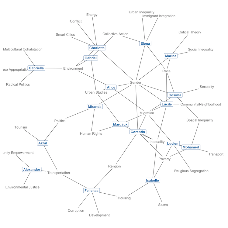
In this graph, students are connected to other students by the keywords that they both listed as research interests. Note that there are a few parts of the graph where it looks like students are directly connected to each other, but this is not the case: in a two-mode network like ours, nodes of the same mode never connect directly to each other.
The network conveys useful information about some keywords, like Gender, Migration and Environment, which act as bridges between several students. It also shows a group of densely connected students on the right, and several students, like Gabriella, Alexander and Felicitas, in peripheral positions on the left, as their choice of keywords more rarely matched with that of other students.
Going back to a one-mode network
Let's now use the information of this two-mode network to connect students to each other. This time, we want to obtain a square, symmetrical matrix that would look like this if there were only 3 students in the class:
$$ \begin{array}{lc} \ B = & \left(\begin{array}{} 2 & 1 & 0 \\ 1 & 3 & 1 \\ 0 & 1 & 2 \\ \end{array}\right) \end{array} $$
This matrix actually contains the same information as the first one that I showed, only in different form: it has the 3 students on both rows and columns, and indicates, for instance, that Student 1 and Student 2 share one common keyword. You can read that information on the first row, second column, or on the second row, first column.
In this matrix, the diagonal indicates the total number of keywords listed by each student (or, if you prefer, the number of keywords that they share with themselves). Since that information is meaningless for our purposes of connecting students to each other, we will later discard it.
We are, however, interested in the other values of the matrix, and even though all these other values are equal to either $0$ or $1$ in my example, that might not be the case in the data, as some students might share more than one keyword with each other.
In other words, what we want here is to obtain a weighted, one-mode adjacency matrix of students, with the weights indicating the number of keywords that they share with each other. Note that we could perhaps find better ways to weigh that matrix, but let's keep it simple and stick with the simplest weighting structure.
How do we do that, starting with the incidence matrix $A$ that we created in a previous section? Here's the trick, in the words of Solomon Messing:
To convert a two-mode incidence matrix to a one-mode adjacency matrix, one can simply multiply an incidence matrix by its transpose.
Or, in mathematical notation, to get the one-mode adjacency matrix $B$ of students, all we need to do is to perform $AA'$ on the two-mode incidence matrix of students and keywords. The only condition for that operation to work properly is that students need to be located on the rows of the incidence matrix, which is the case.
So let's do that, and then convert the result to an igraph network object:
… And we are back with a one-mode network object, only this time, in contrast to the network shown in the previous one, the nodes of the networks are students, not keywords. We could plot the network straight away to show that, but let's add a final twist to our analysis.
Adding clusters, a.k.a community detection
Since what we have in our network are students connected by 0, 1 or more keywords, let's try to group the students together based on that information.
In statistical jargon, finding groups of things based on some properties of these things is called cluster analysis. In network theory, the equivalent is called community detection, and one commonly used method to find communities in networks like ours is called the "Louvain method," named after the university in which it was designed.
It would take too much effort to explain here how the Louvain method works; just take note that it works with networks like ours—that is, one-mode, undirected networks based on a weighted adjacency matrix.
Detecting the Louvain community of each student, i.e. his or her cluster, based on the keywords that he or she shares with other students, takes one line of R code:
Let's now see if the clusters make sense!
Visualizing the one-mode network
Before we proceed to plotting the network, let's also compute the weighted degree centrality of the nodes, which will be useful to show students with less shared keywords in smaller size:
Note that the degree distribution that we have computed here also takes into account the weighted structure of the adjacency matrix that underlies our network.
Let's now finally get to the network plot, with each keyword-clustered group of students shown in a different color:
In this graph, the intensity of the edges (the ties between the students) reflects the number of keywords that they share with each other. The graph uses a different force-directed layout algorithm than the one used in the previous note, but this is only a matter of taste.
Final comments
Looking at this final graph, what can we say about this year's batch of GLM students?
If we trust the method that we used to cluster the students together based on their shared research interests, then Akhil, Alexander and Felicitas should be working together. Similarly, the four students from the "blue" cluster (Gabriella, Gabriel, Alice and Charlotte) should form two student pairs between them.
The results are less obvious for other students, but still, I would expect Mohamed to have paired with either Lucien, Margaux, Corentin or Isabelle, and Marina to have paired with either Elena, Miranda, Cosima or Lucile.
We will see in class if that is what happened in reality, but I can answer that question straight away for readers from outside our class: not at all! This year's GLM students seem to have privileged other forms of ties between them.
The code shown in this note is provided in full in this Gist. If you want to replicate the plot above, you will need to download the data and (install and) load the required packages first.
Update (January 4, 2021): corrected an omission in the code and fixed the last plot to work with recent versions of ggnetwork. Thanks to Piotr Koc for the report.
- First published on September 16th, 2016