ggnetwork: Network geometries for ggplot2
This note is a ~~shameless plug~~ demo of the ggnetwork package, which provides several geoms to plot network objects with ggplot2, and which just got published on CRAN. See the package vignette for a more detailed guide to its functionalities.
Our example data is the most recent version of the Icelandic legal code, which is available as a ZIP archive from the website of the Althing, the unicameral chamber of the Icelandic parliament. The many different parts of the code frequently refer to each other, thereby creating a network of legal cross-references.
We will use Hadley Wickham's dplyr and rvest packages to collect and process the data, the network and sna packages to build the cross-reference network, and the ggnetwork package to plot it, using colors taken from a Wes Anderson palette:
Loading the ggnetwork package will load ggplot2, which we will need to adjust the theme settings of our final plot.
Data collection
Let's start by downloading the raw data. The files that we need to parse within the archive all start with a 4-digit number that indicates their year of adoption, so let's list those files to later read them directly from inside their ZIP archive:
As of time of writing, the data contain 1,513 different legal documents. Icelandic law goes back centuries ago, and some of the legal statutes in our data go back to the 13th century. Most of the texts, however, were adopted in the 20th and 21st centuries.
Note that the Icelandic legal code is versioned by year (or more exactly, by parliamentary session). In a more complex example, we could download all versions of the code since 1995 and plot the network of cross-references between its parts dynamically through time.
Edge list construction
Next, we parse each article to extract its title and date of adoption, as well as any reference made within that article to another part of the legal code. We then remove self-references, clean up the links from their HTML file extension, and weight the resulting edge list by the number of cross-references between each article dyad:
This part of the code creates an edge list of the form $(i, j)$, where legal document $i$ refers to legal document $j$. The last row above shows a cross-reference between the legal document that sets out ministerial areas (Lög 71/2013) and the legal document that details how Iceland organizes its budgetary process (Lög 123/2015):
            i       j     w
        (chr)   (chr) (int)
    1 2013071 2015083     1
    2 2013071 2015085     1
    3 2013071 2015087     1
    4 2013071 2015091     1
    5 2013071 2015112     1
    6 2013071 2015123     1
In a dynamic network, these cross-references would receive a timestamp, and we would be able to show how the network changed both in size and in density through time.
Network construction
Building the cross-reference network from the weighted edge list is very straightforward. The network is directed: article $i$ can reference article $j$ without the reverse being true, and the number of cross-references between them can be—and usually is—asymmetrical.
Once we have obtained the network and weighted its edges, we add Freeman's degree (the sum of each node's indegree and outdegree) to the object as a vertex attribute, as well as the period of adoption of each text--that is, of each node:
The last vertex attribute created above, period, contains roughly equal quantities of legal texts. The boundaries of that attribute show that the cross-references in our data span from the mid-19th century to today:
    [1849,1986) [1986,1997) [1997,2006) [2006,2015]
            214         191         229         233
Network visualization
We now turn to visualizing the network as a ggplot2 object, using the geometries provided the ggnetwork package.
As explained in the package vignette, ggnetwork provides fortify methods for objects of class network and igraph, which means that once the package is loaded, we can pass objects of these classes directly to ggplot2 as if they were data frames. Next, we add one geom for edges, and one for nodes:
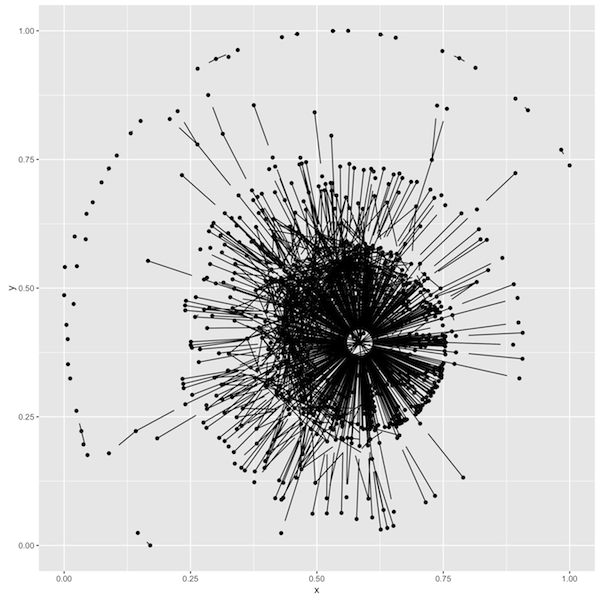
The code above defines the minimal aesthetics required by ggnetwork: the x and y mappings are used for nodes and edge startpoints, and the xend and yend mappings are used for edge endpoints. These mappings work exactly like those of geom_point and geom_segment, as the resulting plot illustrates:

To obtain this plot, the fortify method implemented by ggnetwork has "flattened" the network to a data frame. The data frame contains x and y coordinates for each vertex of the graph (each node of the network), based on a graph layout that defaults to the Fruchterman-Reingold force-directed node placement algorithm.
By default, ggnetwork "shortens" the edges of directed graphs in order to leave a bit of space to draw directed edge arrows before they "reach" their target nodes. It also turns edge and vertex attributes into columns of the fortified data frame, which means that our degree vertex attribute is available through aesthetic mappings.
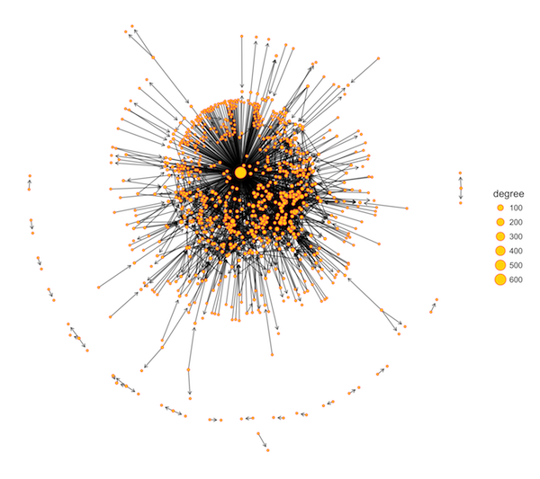
Let's play a bit with the aesthetics of the plot by reducing the default shortening effect of the edges, adding edge arrows, making the edges semi-transparent, and sizing the nodes proportionally to their Freeman's degree. We will also use a custom point shape to illustrate how to draw vertex borders:

The theme_blank() object is a minimalistic ggplot2 theme that removes pretty much everything (axes, ticks etc.) from the plot. What this last example shows is that we can manipulate our network plot exactly like any other ggplot2 object, so let's show a final example of the kind of visualization that we can get from ggnetwork:
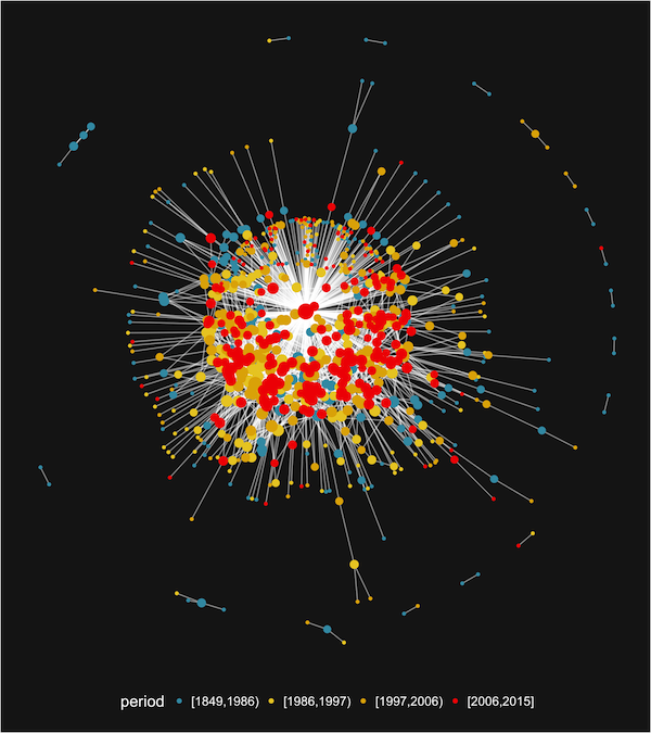
This code shows the same (unweighted) network of all cross-references that we found in the Icelandic legal code, minus the edge arrows, and with additional colors to distinguish older from newer legal documents. The highly central node in the middle of the plot is the previously mentioned Lög 2013/71 text:

This note updates an example featured in the vignette of the ggnet package, which offers a different method to plot network objects with ggplot2 (read more about it in this other note). Its code is available from this Gist.
Update (May 17, 2016): the ggnetwork package got featured in the R World News - Episode 1 podcast by Bob Rudis and Jay Jacobs. See this blog post for more details about the podcast.
- First published on March 28th, 2016